From the quantum world to the guy next door (part 1)

This post will be a little more technical than the usual ones. Nonetheless, I believe there ia "market" for it: students who are just learning quantum mechanics and might require to dispel much of the baloney that is told about the quantum weirdness. Recently I was discussing with one of the cobloggers of astronomers in the wild about some limerick from David Morin's mechanics book:

When walking, I know that my aim

Is caused by the ghosts with my name.

And although I don't see

Where they walk next to me,

I know they're all there, just the same.

This is mentioned just as some side note when discussing the stationary action principle, specifically, in the context of learning if there is a deep reason behind it. The stationary action principle says that the quantity S, called the action and given by

\[ S= \int_{t_a}^{t_b} dt\ L(x,\dot{x};t) \]

should take a stationary value. That means that from all possible paths involved in getting from a to b, a classical particle will take the path in which the action takes a minimum value (well, actually a stationary one, usually the minimum). This is the principle behind classical mechanics. The motion of everything we can see around us, including the stars in the sky or matter around a black hole follow from this principle.

Hence, it would be great to know if there is a reason behind this principle. Well, yes, there is. It is deeply rooted in quantum mechanics and its essence is captured in above's limerick.

So, the purpose of the few next posts will be to see how we can pass from the quantum description of the world to the kind of phenomena we observe everyday when dealing with baseballs, pulleys and all that.

This is not a trivial question, every experiment has confirmed the validity of quantum mechanics as the correct description of our world but it is in stark contrast with the intuition we have all developed from observing microscopical objects all our life. Nonetheless, at first glance, both descriptions are radically different. To see how weird the quantum behavior is for us, macroscopic beings, let's consider one situation that shows most of the quantum subtleties: the double slit experiment.

Consider some particles source S, placed at a point A. In front of it, we place a screen C with two slits in it. Hence, we expect that any particle arriving to a screen at the point B where the arrival of electrons is measured must pass through one of the slits. This configurations is shown below.

Well, if we do this experiment with marbles, baseballs, grains of sand or any other classical object coming out of the source S, then the outcome will be just what we expect. Namely, if we shut one of the slits, then the distribution of arriving marbles at B will be peak just in front of the open slit. The resulting distribution of arriving marbles at B when both slits are open is just a sum of the peaks produced by the particles entering through each slit. This is shown below.

Here, the outcome of the double slit experiment with classical particles is shown. If we shut one slit, we get one sharp distribution (shown in blue). The outcome with both slits open is just the sum of the two peaks and it is shown in red.

There is a second classical object that we can throw against our screen at C: waves. So, lets imagine that we place the whole setup in a pool and the source at A stirs the water a little bit so it create waves. In a realist experiment, we should place S very far from C so we can have some nice plane waves arriving at C, but ignore such nuances for our purposes. When the incoming wave arrives to C, each slit will act as a new wavefront and produce an outgoing wave. Since we have two slits, the outgoing waves will be out of phase from some parts and in phase for others. This is better seen in the picture below.

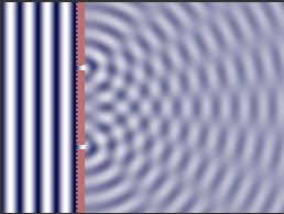
The darker zones correspond to places where destructive interference happens, namely where the waves are completely out of phase and cancel out. On the other hand, clear zones are where waves are in phase and constructive interference happens. The outcome of all this, is that the distribution at B will be different from the one we got using marbles as we now have some interference pattern, as shown below.

As you can see, we now have many peaks and actually the biggest one is in front of a closed part of the screen C ! This is just the result of the way waves behave: they can add or subtract from each other in stark contrast with marbles as we do not expect one marble to cancel another!

So, if an electron behaves exactly as a marble we expect that the chance of arrival at some point x of the target B will obey two simple rules:

1. Each electron which passes from the source S to some point x in B should go through either hole 1 or 2.
2. The chance of arrival to x is the sum of two parts: P1 the chance of arrival coming through hole 1, plus P2; the chance of arriving after coming through hole 2.

I repeat, this is the case for classical particles. Even in classical mechanics we can get a different behavior by using waves, as illustrated above. Now, we use to imagine electrons as lil' charged things and with a big degree of naivety we would expect these two rules to extend to electrons.

Well, what happens when we use electrons? It turns out that we get a distribution identical to the one we get from waves! This is a good place to stop today, but nonetheless I should tease you a little.

The questions that arise immediately are: is the electron a wave? If so, how can we reconcile that with our intuition that it should pass through one hole? how can we measure that? As of now, we could actually say that the electron is indeed a wave. Nonetheless, that contradicts our experience of electric charge as a flow of electrons, which has proved to be extremely successful. Additionally, when using electrons to strip electrons from some metal the behavior is consistent with particles (its analog with photons is the well known photoelectric effect). Actually, all the subsequent discussion for the quantum case can be carried as well with photons. This kind of behavior with electrons behaving as confused teens not making their mind about being particles or waves is usually stated as the wave/particle duality. Hopefully, by the end of this series of posts you will agree with me that such duality is a rather childish way to describe things: electrons are particles, which get their peculiar behavior due to the way probabilities/amplitudes add. Furthermore, the mechanism to get the amplitude will lead us directly to the classical world with which we are all so familiar.

Besides, now that we can not use the two rules stated above, what rules should we use to calculate the distribution at B? This last question is essential: the big difference between the classical and quantum world is in the way we calculate probabilities. That is the topic for the next post. Meanwhile, you can read what happened when this experiment was performed in 1998 by E. Buks et al.

For all you able to read spanish, I decided to continue this "story" in my spanish website: sinédoque. This was due to the capabilities of blogger which were too meager at the time, specially regarding mathematical expressions. I have just implemented a new system on this blog so maybe some more "math heavy" posts will appear here in the future. Keep tuned.

The Towers of Hanoi

I don't know why but I recently came back to this old, interesting little problem. For those not familiar with the puzzle, here's an excerpt from Wikipedia:

[The Towers of Hanoi puzzle] consist of three rods, and a number of disks of different sizes which can slide onto any rod. The puzzle starts with the disks in a neat stack in ascending order of size on one rod, the smallest at the top, thus making a conical shape.

The objective of the puzzle is to move the entire stack to another rod, obeying the following rules:

• Only one disk may be moved at a time.
• Each move consists of taking the upper disk from one of the rods and sliding it onto another rod, on top of the other disks that may already be present on that rod.
• No disk may be placed on top of a smaller disk.

Here's an image of how the initial configuration looks like with 8 disks (also from Wikipedia):

Also, here's an applet of the puzzle so you can try to solve it yourself: MazeWorks - Tower of Hanoi. Try with 3, 4 and maybe 5 disks, and see if you can solve it with the fewest number of moves.

You'll notice that, according to that applet, the minimum number of moves for the puzzle with N disks seems to be 2^N-1. The other day it occurred to me that this can be proven by mathematical induction easily, and that the procedure for doing so is actually the recipe for a recursive algorithm to solve the problem. I'll talk about these two items separately.

Proof that it takes 2^N-1 moves to solve the puzzle.

We want to prove that a solution to the Towers of Hanoi problem requires 2^N-1 moves, where N>=1 is the number of disks to move. Let's proceed by mathematical induction.

1) Base case: we prove the claim is valid for N=1.

If there is one only disk, moving it to the correct peg requires (trivially) a single move. And 2^1 - 1 = 1, which show what we want to prove is true for the base case.

2) Induction Hypothesis: we assume the claim is valid for N=k, where k >= 1 is some number.

This assumes that the solution to the k-disk problem takes 2^k - 1 moves. That is, we assume it takes 2^k - 1 moves to transfer k disks from one peg to an empty peg, using a third empty peg as auxiliary. Note that because of the rules, an "empty peg" is equivalent to "a peg containing one or more disks that are all larger than the disks we're moving".

3) Prove the claim holds for (k+1) disks: we must show that if the induction hypothesis is true, then we can prove that the claim is true for the (k+1)-disk problem as well.

In other words, we want to show that if it's true that the k-disk problem requires 2^k-1 moves to solve, then the (k+1)-disk problem requires 2^(k+1)-1 moves to solve.

So we want to solve the (k+1)-disk problem. Let's call the peg on which the disks initially reside the S (source) peg, the peg to which we want to transfer all the disks the D (destination) peg, and the third peg the I (intermediary) peg, which we'll use as auxiliary peg during the process. Then, we proceed as follows:

1. Move the upper k disks from the S peg to the I peg. This is possible since we assumed it in the induction hypothesis, which also establishes doing so takes 2^k - 1 moves. This leaves the largest disk alone on the S peg.
2. Now that it's possible, move the largest disk from the S peg to the D peg. The disk is now in its final position, so we don't have to move it again. This takes 1 move.
3. Move the k disks that were on the I peg to the D peg. Again, by induction hypothesis, this takes 2^k - 1 moves. It doesn't matter we're moving the disks to a non-empty peg, since the disk on the D peg is larger than any disk we're moving, and hence doesn't interfere with the task. The S peg is used as auxiliary peg in this process. After this, the problem is solved, for all disks lie on the D peg.

So what was the total move count? In step i), we used 2^k-1 moves, in step ii) a single move, and in step iii) 2^k-1 moves again. The total:

Moves = (2^k-1) + (1) + (2^k-1) = 2*(2^k) + (1-1-1) = 2^(k+1) - 1

And so, we have proved that if it takes 2^k-1 moves to solve the k-disk problem, then it takes 2^(k+1)-1 moves to solve the (k+1)-disk problem. This, together with the base case whose validity we verified in the first step, makes the claim valid for all N. Q.E.D.

Optimality

Note, however, that at first this proof does not guarantee this is the optimal number of moves needed to solve the problem, only that the N-disk problem can be solved with 2^N-1 moves. Luckily, it seems I can justify the optimality of the solution formally.

Consider the following modified proposition, which we'll prove by induction too: "It takes 2^N-1 moves to solve the N-disk problem, and this is the minimum number of moves of any solution". This is trivially true for the base case (N=1).

To prove the induction step, consider the following argument. We want to show that solving the (k+1)-disk problem requires a minimum of 2^(k+1)-1 moves.

But consider that no matter how you solve the problem, at one point you'll need to move the largest disk to the D peg. Since the largest disk cannot be placed on top of any other disk, this means that the remaining k disks must be on the I peg when this happens. There is no other way this could be. So any solution strategy, no matter what is is, must pass through this common state.

Now, by the (modified) induction hypothesis, moving k disks from one peg to another is done optimally in 2^k-1 moves. So putting the puzzle in the configuration required to move the largest disk to the D peg requires a minimum of 2^k-1 steps. Similarly, after the largest disk is moved to the D peg, transferring the remaining k disks to the D peg also requires a minimum of 2^k-1 steps.

Finally, the middle step, moving the largest disk to the D peg, is trivially optimal, since we're moving a single disk.

With this, we prove that if the solution of the k-disk problem requires a minimum of 2^k-1 moves, then the solution of the (k+1)-disk problem requires 2^(k+1)-1 moves, and that it is also the minimum number of moves.

The uniqueness of the optimal solution is also proved with the same argument, since moving a single disk (both in the base case and in moving the largest disk to the D peg) is both optimal and the unique way to do it.

Solution Algorithm

A nice thing of this proof by induction is that it naturally produces a recursive solution algorithm. Basically, we define a function, let's it call it Solve(n, A, B, C), that moves n disks from peg A to peg C, using peg B as intermediary. The function is defined recursively following the logic of the proof above (Python pseudocode):

def Solve(n, A, B, C):
if (n==1):
A.transferTo(C)
else:
Solve(n-1, A, C, B)
A.transferTo(C)
Solve(n-1, B, A, C)

This is almost full Python code; it's only missing the data structure definitions needed to handle the disks and pegs. But it shows the heart of the algorithm. Note how the function calls itself recursively twice: first in a series needed to move the (n-1) disks to the intermediate peg, then in a second series to move the (n-1) disks onto the final peg. In each call, the peg order is changed to reflect which pegs are source, destination and intermediate.

You can get the full Python code here.

LHC alarmism debunked

I just attended a seminar by Michelangelo Mangano titled "Black holes at the LHC: safety and society". While of course the bottom line was that there is no real risk of the LHC destroying the universe it is still worthwhile to discuss it a little bit.

So, a little compendium of why you shouldn't be scared of LHC produced black holes:

• LHC is almost surely not likely to produce black holes, simple as that, most of the models predicting such scenarios work with additional dimensions and require a higher center of mass energy than would be available at LHC. Anyway, there are indeed some scenarios where black holes can indeed produced at LHC, they are not very plausible but a case can be surely made from them.
  
• Black holes are unstable: Black holes decay via Hawking radiation. Particles can be created out of "nowhere" in the vacuum, a rather sloppy argument essentially says that the uncertainty principle allows particles to pop out of nowhere as long as the energy loan required to create them is payed really fast. Now, consider one of this virtual particles being created just outside the black hole and the other one just inside of the black hole. The net effect for an observer outside the black hole is that black hole is radiating, in the process the black hole is loosing mass that is just escaping in this radiation. This radiation is not only electromagnetic, in principle a black hole can radiate anything.
  This makes the black hole to "evaporate" as it looses mass via radiation, it turns out that the lifetime of a black hole is proportional to its mass. For black holes with really small mass, like the ones speculated to be produced at LHC this yields out such a short lifetime that there is not a reason to worry at all.
  We can now be cynical and say that QFT in curved spacetime (the fancy name for the framework used to calculate this kind of things) is not really experimentally established, maybe there is something wrong with it and black holes could be stable, then you should consider that...
• Black holes produced in particle collisions are charged: Collisions at hadron colliders happen between the charged components of protons and conservation of charge requires that the final product (in this case a black hole) remains charged. Any charged particle, even a microscopic black hole interacts with matter in a way that has being throughly studied and is summarized in the so called Bethe-Bloch equation for the range of energies likely involved in the LHC. The result is that the black hole will just radiate all its energy away in a short distance. But hey, what if we are somehow missing something in the creation of microscopic black holes and it is possible to produce stable and neutral black holes? This looks extremely unlikely but lets go ahead and see what can happen if they are indeed produced.
• Accretion rates from microscopic black holes are negligible: Lets say we have a slow moving, stable and neutral black hole. Can it eat the Earth and cause all other kinds of havoc? Well, if we model mass infall into a black hole via Bondi accretion (a fancy name for spherical accretion) it turns out that to gain a considerable mass, say 1 ton, a huge amount of time is required. Right now I don't remember now the exact number but it was of the order of a thousand millions of years. If a predator capable of running at most a 1mm per year is chasing you with bad intentions you wouldn't be scared, would you?

Well, despite this arguments there is still people around trying to halt LHC and the issue has even been brought to court, where it has always been dismissed based on technicalities, mostly because the LHC is out of jurisdiction of the court.

So, why I am telling you all this? Well, wait for tomorrow...

Create wallpaper slideshow in Ubuntu 9.10

First of all, happy new year! Nothing like the morning of a new year to be messing around with Linux and Python!

One of the new things in Ubuntu 9.10 is that you can now use a wallpaper slideshow for your desktop, which will cycle your desktop wallpaper at regular intervals from a selected pool of wallpapers. The default Ubuntu 9.10 comes with a space-themed wallpaper slideshow, but there is apparently no option to create your own ones. However, the configuration is stored in plaintext XML files, one in /usr/share/gnome-background-properties and the other in the corresponding directory where the images are stored, in /usr/share/backgrounds.

The following Python script will automatically create these two XML files so that you can set a wallpaper slideshow with the images of your preferences.

Slideshow Builder script
(Right-click and select "Save Link As..", or the equivalent in your browser).

Here's the instructions. You will need root access since the directory where you're doing the operations, /usr/share/, is owned by root. Simply use sudo (or sudo -i if you're lazy).

1) Create a directory in /usr/share/backgrounds with the name of your slideshow. For instance, if the desired name is 'space', the dir should be called '/usr/share/backgrounds/space/'.

2) Copy all the wallpaper images to that folder. The supported formats are jpg, png, gif and bmp.

3) Run the Python script in the images directory. This will automatically create two xml files: one in the (current) images directory, and another one in /usr/share/gnome-background-properties.

4) That's all! You can now select the slideshow in the Gnome wallpaper selection interface.

A sample usage of the script is shown in the following image:


And the slideshow now appears in the desktop Background selection screen:

Update: I've fixed the dead link to the script.